Consider the Lotka-Volterra predator (y) prey (x) model:
Solution curves for various initial populations are plotted below:
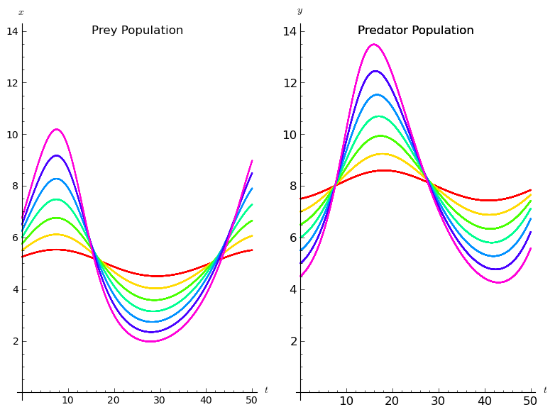
(x(0), y(0)) = (5.25, 7.5), (5.5, 7), (5.75, 6.5), (6, 6), (6.25, 5.5), (6.5, 5), (6.75, 4.5)
Another way to visualize the solution curves is plotting the trajectories in the phase plane. This is called the phase portrait.
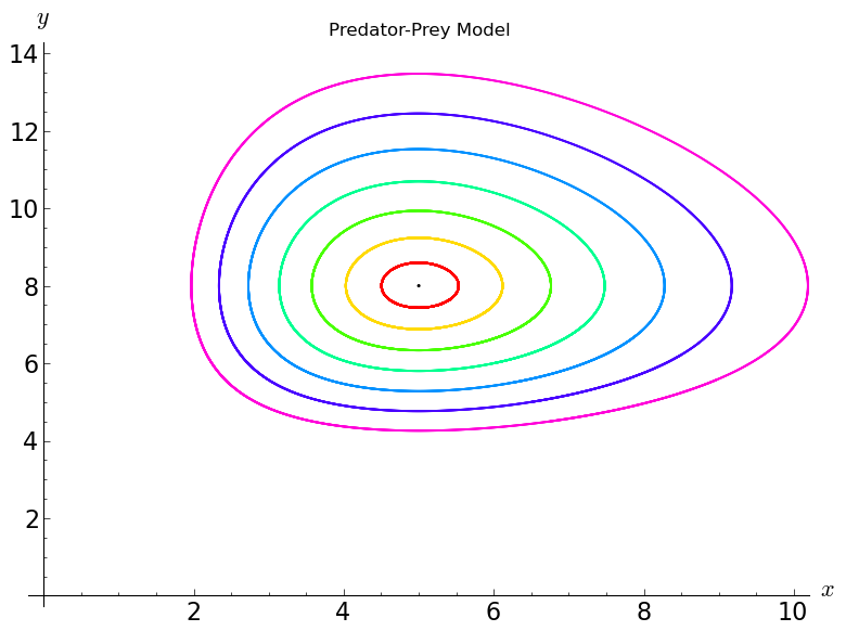
Notice the critical point (5,8). The constant functions x(t) = 5, y(t) = 8 form a solution to the system.
Images generated by sage.