Driven Damped Motion

Driven damped motion of a mass m is modeled by the 2nd order ODE:

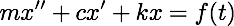
where x(t) is the distance from equilibrium, c is the damping constant, k is the spring constant and f is an external driving force. We divide by m and write:

$x'' + 2\lambda x' + \omega^2 x = F(t)$

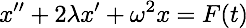
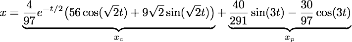
where 2λ = c/m, ω² = k/m and F = f. The general solution breaks up into two pieces, the complementary and particular:

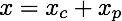
where x_c (the complementary solution) is transient, in other words satisfies x_c(t) → 0 as t → ∞. Hence we see that for any initial conditions the long term behavior of x is just x_p. This term is called the steady-state term.

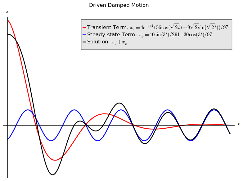
The graph below plots the solution and the decomposition into transient and steady-state terms for the IVP:

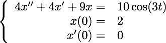
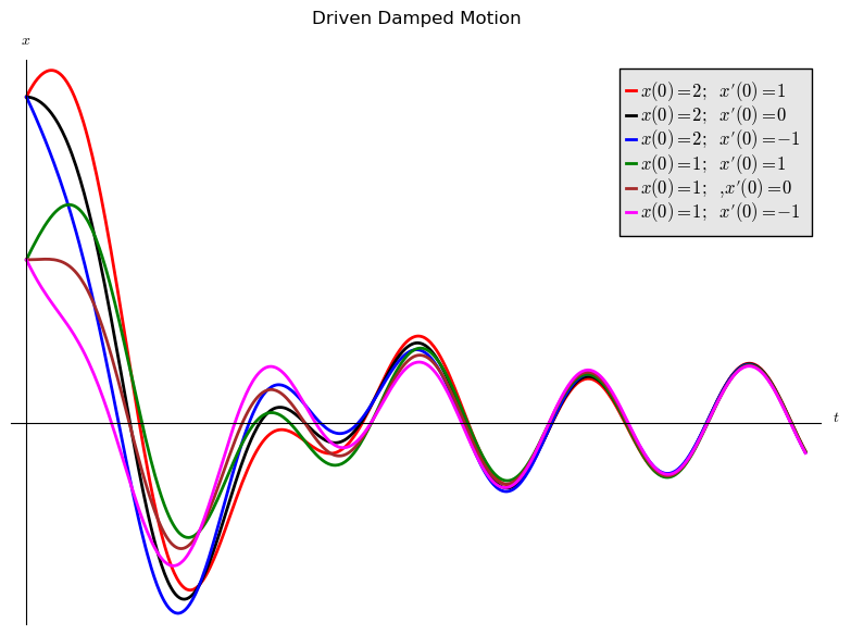
Changing the initial velocity changes the transient term, but not the steady-state term. The graph below shows the solution curves that result when the initial conditions are altered. Notice that eventually the graphs looks the same.

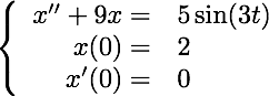
When f (t) = F₀ sin(ω₀ t), where ω₀ = (ω² - λ²)^½ is the natural frequency of the system, resonance can occur. This is the phenomenon by which the oscillations grow without bound, potentially ripping the system apart.

For example, the following IVP models a driven undamped system where the driving frequency equals the natural frequency:

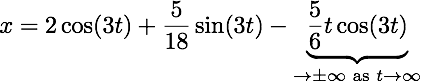
Images generated by sage.